
Our favorite operational amplifiers (op amps) originally served to perform arithmetic operations on voltages: addition, subtraction, multiplication, and division. These capabilities let us amplify weak signals, for example, in an automatic high-beam controller.
When driving on an unlit road at night, we use high beams to spot hazards early and respond in time.

However, an oncoming driver may also have their high beams on. The resulting glare can impair both drivers’ vision and even cause a crash.
A simple automatic controller detects oncoming headlights with a light sensor and briefly switches our headlights to low beams, reducing glare for the other driver.
This gives the two vehicles time to pass each other. The controller then restores the high beams so we can see farther down the road.
In this design, the sensor is intended to respond to bright oncoming headlights rather than other light sources along the road, including the taillights of vehicles ahead.

For this project, we’ll use a photovoltaic (PV) cell, similar to those in solar power systems and solar-powered garden lights, rather than a photoresistor or photodiode.

To amplify the PV cell’s signal, we’ll use a circuit called an instrumentation amplifier. It has two inputs, noninverting and inverting, and amplifies the voltage difference between them by a set gain.
We’re already familiar with op amps, which have the same two inputs. With negative feedback and operation within its linear range, an op amp adjusts its output to keep its input voltages nearly equal.
We can build an instrumentation amplifier using three op amps, as shown in the schematic.
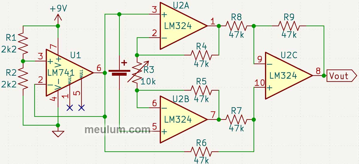
An additional op amp, U1, provides a buffered midpoint reference, or virtual ground, at half the supply voltage.
In our case, this is 4.5 V, since a regulated 9 V supply powers the PV cell’s amplifier circuit.
R1 and R2 have equal resistance, so the voltage drop across each divider resistor is the same: each drops half of the 9 V supply voltage.
The instrumentation amplifier, with its three op amps and seven resistors, may look complicated. But two key principles make its operation easier to understand.
First, an ideal op amp draws no input current. In our idealized analysis, current flows through the resistor network without entering the op amp inputs. There are four op amp outputs in this part of the circuit.
The PV cell’s negative terminal connects only to U2B’s noninverting input, whose input resistance we assume to be infinite. The instrumentation amplifier therefore draws no current from the PV cell in this ideal model.
Second, the amplifier stages under discussion use negative feedback. As noted above, we treat their input voltages as equal in the ideal model, provided the amplifiers remain within their linear operating range.
To simplify the calculations, we’ll treat virtual ground as 0 V. We’ll denote the input voltage - the PV cell’s electromotive force (EMF) - as −Vin because the cell’s positive terminal connects to this reference point.
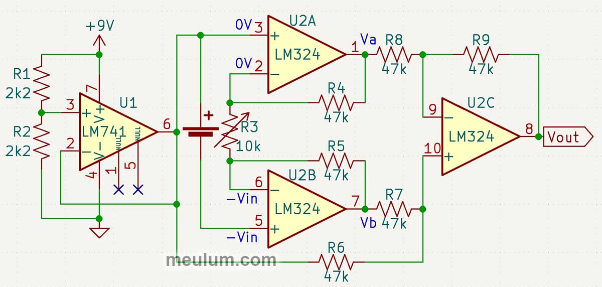
The output voltage at U2C is Vout. To find it, we first need to calculate Va and Vb at the outputs of U2A and U2B.
We have three resistors in series: R4, R3, and R5. We know the voltages at both ends of R3: 0 V at the top and −Vin at the bottom.
The fixed resistors in this instrumentation amplifier have the same resistance, 47 kΩ; R3 sets the gain. We’ll use R, without a subscript, for the fixed resistance and apply Ohm’s law to each of the three series resistors. The same current, Iab, flows through them from U2A’s output to U2B’s output.
Iab = (Va − 0)/R = Va/R
Iab = [0 − (−Vin)]/R3 = Vin/R3
Iab = (−Vin − Vb)/R = −(Vin + Vb)/R
Vin(1 + R/R3) = −Vb
Therefore:
Va = Vin × R/R3
Vb = −Vin(1 + R/R3)
We now have a voltage amplifier with a differential input and a differential output. Its output voltage difference is:
Va − Vb = Vin × R/R3 + Vin(1 + R/R3) = Vin(1 + 2R/R3)
The circuit multiplies the differential voltage at the noninverting inputs of U2A and U2B by (1 + 2R/R3). It therefore performs analog multiplication by a set factor.
At R3’s maximum resistance of 10 kΩ, the minimum gain is:
1 + 2 × 4.7 = 10.4
At R3 = 1 kΩ, the gain is 95. At R3 = 100 Ω, it is 941.
Instrumentation amplifiers can amplify microphone signals, providing high gain that a single variable resistor adjusts over a wide range. They also reject common-mode interference.
To process the PV cell’s signal further, we need a single-ended output rather than two differential output voltages. The third op amp, U2C, provides this output.
Negative feedback through R9 keeps U2C’s two input voltages equal in our ideal model. We’ll call this voltage Vc.
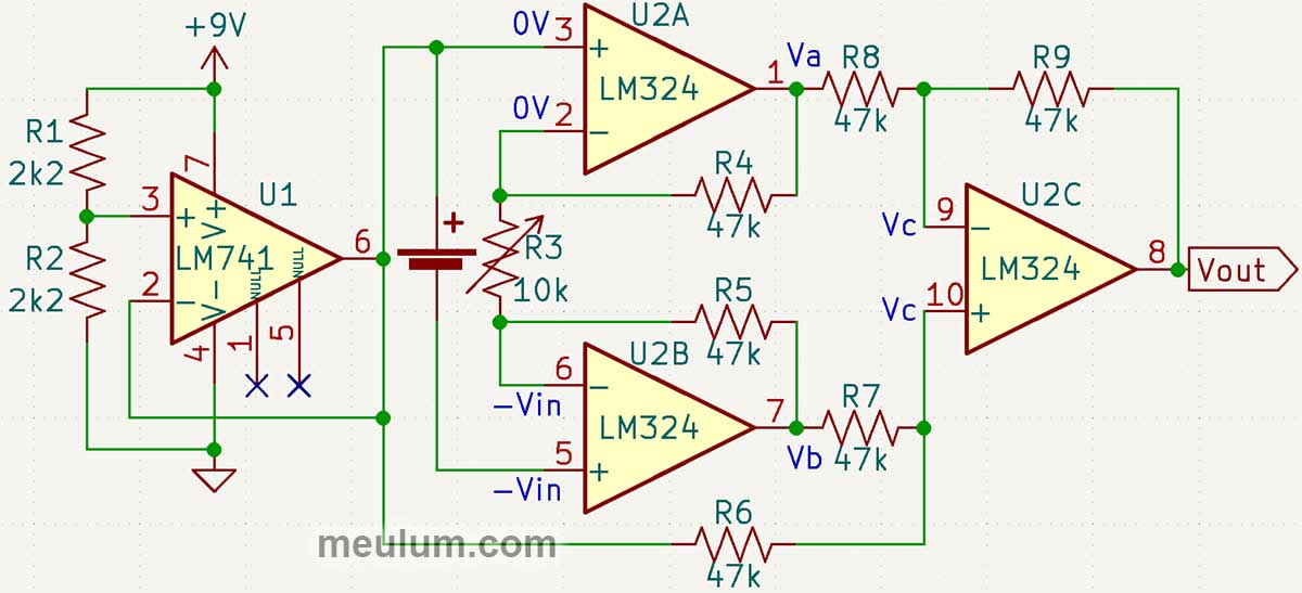
Here, we have two currents: one flows through R9 and R8, and the other through R7 and R6. Since all four resistors have equal resistance, we can write:
Vout − Vc = Vc − Va
Vout = 2Vc − Va
Vb − Vc = Vc − 0
Vb = 2Vc
Vout = Vb − Va
Substituting the values we calculated for Va and Vb gives:
Vout = −Vin(1 + 2R/R3)
We used virtual ground as our 0 V reference. Relative to the negative supply rail, the output voltage is:
Vout = 4.5 V − Vin(1 + 2R/R3)
We’ve multiplied the PV sensor’s voltage by a negative factor and added 4.5 V. We can also describe this as multiplying Vin by a positive gain and subtracting the result from 4.5 V. We’ve built a tiny analog computer.
The fourth operation, division, takes just two resistors. Voltage dividers provide both the midpoint reference for virtual ground and the reference voltage for comparator U2D, which receives the instrumentation amplifier’s output, Vout.
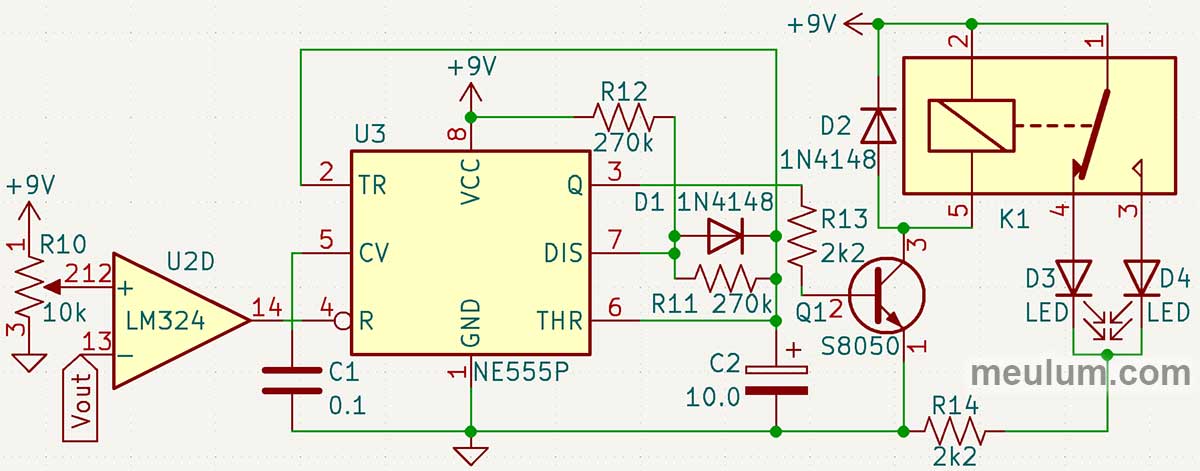
Potentiometer R10 adjusts the divider ratio and, in turn, the comparator’s switching threshold.
The fourth op amp in the LM324 serves as the comparator. It has no negative-feedback loop. When the noninverting input voltage exceeds the inverting input voltage, the output goes high. When the input relationship reverses, the output goes low.
The comparator’s output drives the reset input of a 555 timer operating in astable mode. When little light reaches the sensor, the timer stays in reset, the transistor is off, and LED D4 lights up. In the model, D4 represents the high-beam lamp; an actual headlight would require a suitable lamp or LED-driver interface.
Bright oncoming headlights cause the instrumentation amplifier’s output voltage to drop, switching the comparator and releasing the 555 timer from reset.
The transistor turns on, the relay energizes, and D3 lights up in place of D4. D3 represents the low-beam lamp and stays on briefly, giving the vehicles time to pass.
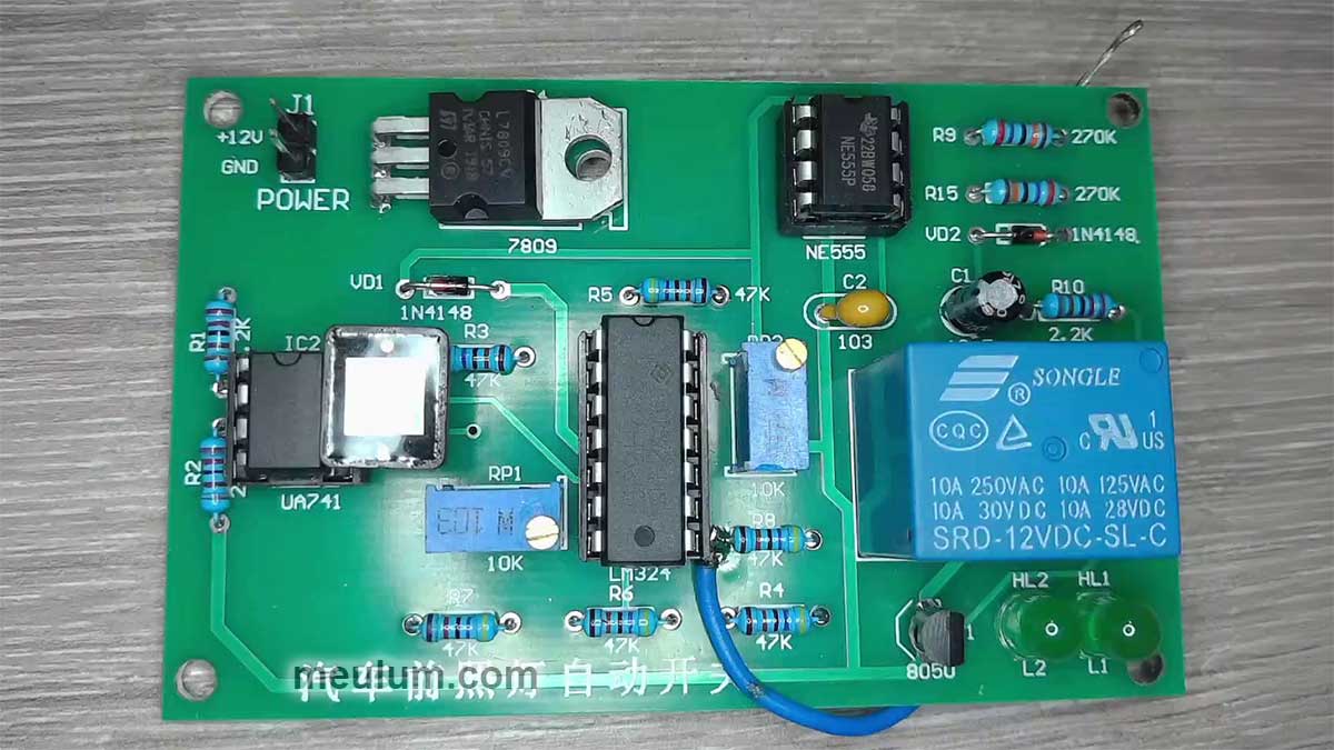
When the bright light no longer reaches the sensor, the controller immediately restores the high beams. If the PV cell remains brightly illuminated for longer, this circuit cycles between high and low beams, periodically illuminating the road farther ahead.


